In this article, different practical methods to reduce the hydraulic demand of fire sprinkler systems are investigated. The example below illustrates how several design decisions influence the final system demand.
Project Information
- Occupancy hazard classification: OH2
- Area: 200 ft × 130 ft
- System type: Wet pipe
- Sprinklers: Upright spray sprinklers, standard response, K5.6
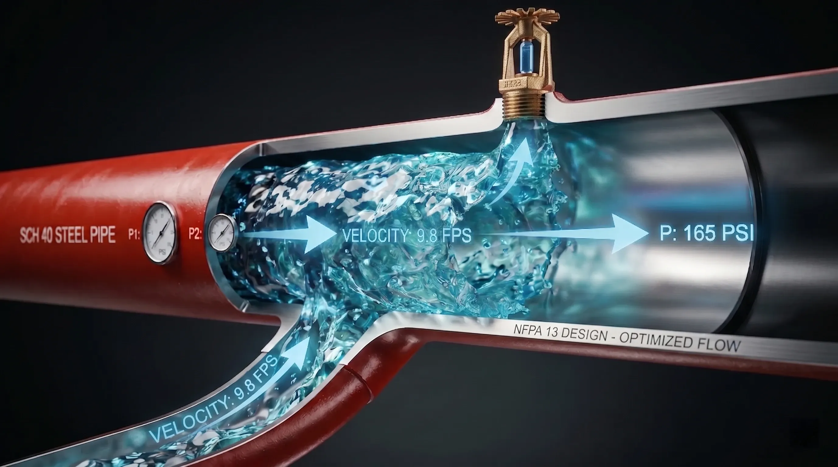
- Pipe type: Black steel, Schedule 40
- Sprinkler coverage: 13 ft × 10 ft
- Branch line elevation: 10 ft
- Cross main elevation: 9 ft
- Ceiling height: 10 ft
- Hose stream allowance: 250 gpm
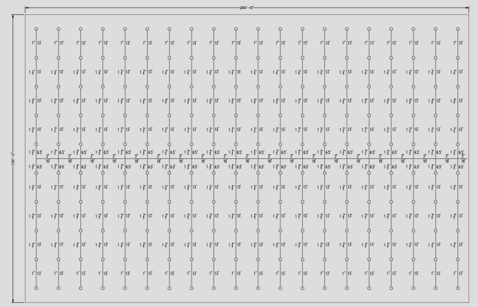
Selecting the Lowest Point of the OH2 Curve
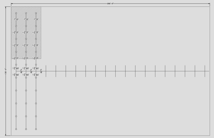
According to NFPA 13 (2022), selecting the lowest point of the OH2 density/area curve results in a density of 0.2 gpm/ft² with a design area of 1500 ft². In this example, the design area includes 12 sprinklers.
592 gpm at 77.4 psi
Upsizing the Pipes
Increasing pipe diameter reduces friction loss in the piping network. According to the Hazen–Williams equation, friction loss is highly dependent on the internal pipe diameter (power of 4.87). Therefore, even a small increase in pipe diameter can significantly reduce pressure demand.
589 gpm at 65 psi
Pipe Wall Thickness
Pipe wall thickness directly affects internal pipe diameter. Thinner pipes increase the internal diameter and therefore reduce friction loss.
591 gpm at 71.3 psi
Quick Response Sprinklers
Quick response sprinklers can significantly reduce system demand because NFPA 13 allows a reduction in the design area when they are used. For a ceiling height of 10 ft, the design area may be reduced by 40%.
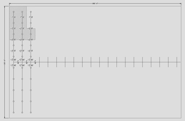
449 gpm at 52.8 psi
K-Factor of Sprinklers
The sprinkler K-factor defines the relationship between pressure and flow rate. A higher K-factor allows the same discharge flow at lower pressure.
Example comparison for a target discharge of 30 gpm:
- K5.6 sprinkler requires 28.7 psi
- K8.0 sprinkler requires only 14.1 psi
620 gpm at 73.7 psi
Velocity Pressure
Velocity pressure is typically ignored in sprinkler hydraulic calculations. However, it can become relevant when pipe diameters are small and flow velocities increase.
584 gpm at 76.3 psi
Upper Point of the Density/Area Curve
Selecting the upper point of the OH2 density/area curve (0.15 gpm/ft² over 4000 ft²) reduces the pressure required at individual sprinklers but increases the overall system flow demand.
732 gpm at 69.5 psi
Smooth Pipes
Smooth pipes such as copper Type M have a higher Hazen-Williams coefficient (C = 150) and a larger internal diameter, which reduces friction loss.
585 gpm at 65.9 psi
Darcy–Weisbach Equation
For smoother pipes, the Darcy–Weisbach equation may produce more accurate results than Hazen–Williams. However, it requires iterative calculations involving pipe roughness and Reynolds number.
584 gpm at 65 psi
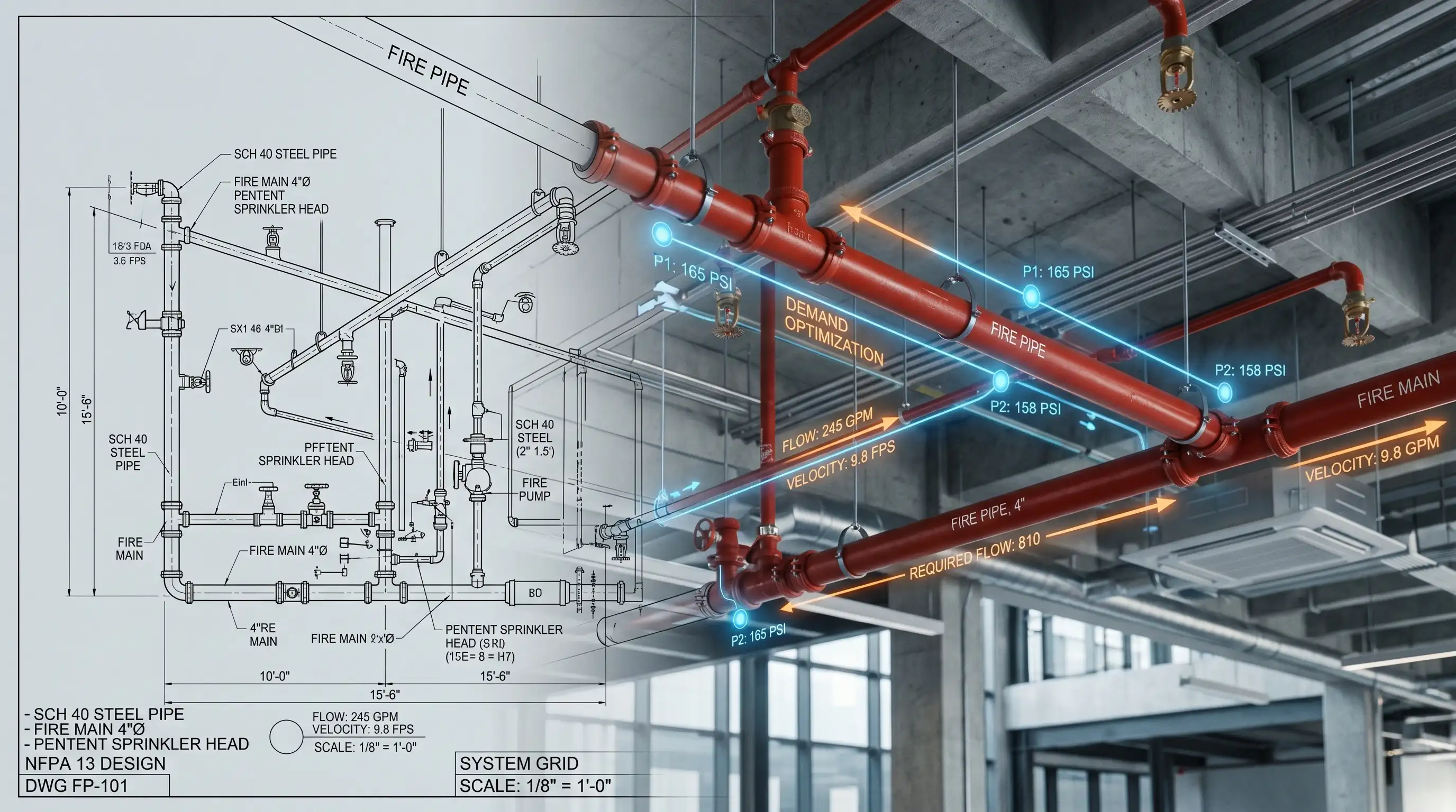
Gridded Piping Configuration
A gridded piping layout is one of the most effective methods to reduce hydraulic demand because water can reach sprinklers through multiple flow paths.
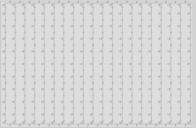
565 gpm at 48.3 psi
Conclusion
Several design decisions can significantly affect the hydraulic demand of sprinkler systems. Designers must evaluate all project conditions and select the most cost‑effective combination of pipe sizes, sprinkler types, and piping configurations.


No comments yet. Be the first to share your thoughts!